In this blog, I try to first introduce variational methods in general and then connect it with the variational methods in machine learning thereby giving a more complete picture. Another experiment I do here is to present this material in the form of dialouges. In that, I burrow Douglas Hofstadter’s style (actually the dialogue between the master and disciple is quite common in philosophy, but the way Hofstadter used fictional characters in the dialogue –in his book Godel Escher Bach– gave an amusing feel!; hence this format).
Po: Master Oogway, I see variational everywhere: Variational Bayes, Variational Autoencoder. What does variational mean?
Oogway: In short, variational methods or principles are techniques that optimize over a space of functions. It is analogous to ordinary optimization problem where we have an objective function that we try to optimize with respect to a variable. Variatinal methods use the same idea, with one main difference: in variational methods, we try to optimize with respect to a function. The idea probably emerged from Physics and had impacts in mechanics, statistical Physics as well as Quantum mechanics.
Po: Hmm, derivative with respect to a function? How do you do that? What do you take derivative of? Another function?
Oogway: Derivative of a real number with respect to a function. It will become clear if you are familiar with the idea of a functional. Just like a function takes in a vector and spits out a real number, a functional takes in a function and spits out a real number. So, a functional is a function of functions. If it helps, you can think of a space of functions as a regular 2D space, just imagine that each point denotes a function instead of a finite dimensional vector. Then, the functional is a map from this space to the real number line. This may be mathematically represented as $L:\mathcal{F} \to R$, where $\mathcal{F} $ denotes space of functions, $R$ denotes real line and $L$ denotes a functional. So, variational methods are those methods that optimize the functionals with respect to functions.
Po: Ahh, I see. That is quite interesting. But, how exactly is that done?
Oogway: How do you think it would be done? Imagine you are a mathematician of that era. How would you go about solving optimization like this?
Po: Ahaha. Umm, I don’t know! What do I know? All I know is that if you need to optimize, you take derivative and equate to zero :D But, I guess this would not be that simple.
Oogway: There are multiple ways. But, the idea that you just mentioned is also a valid idea. It’s just that you need to define derivative with respect to a function. More importantly, you need to think deeper what taking a derivative with respect to a function means and what equating it to zero means. You see, if you were a mathematician of that era, you would be successful if you thought at a slightly deeper level and persevered a little longer.
At that time, there were people who did think deeper and did persevere and came up with something called calculus of variation which expands the idea of taking derivative and generalizes it to take derivative of a functional with respect to a function. Whenever you need to do extend something fundamentally and develop an entirely new way of doing things, you start from the first principles. So, you go back to ordinary calculus and try to understand what it means to say that the derivative of a function with respect to a variable is zero. Imagine a convex function, say $y=(x−1)^2$. You know the minima is the point $x=1$ where the derivative is zero. But, what this essentially means is that if you perturb x by a small quantity, say $\epsilon$, around $x=1$, then $y$ would not change too much. However, if you do similar things around other points, the change is $y$ is large. Now, we see the core idea. The idea is to make small perturbation in $x$ and see the change in $y$. The optimal point is the one where if you change $x, y$ would not change at all.
Now, we can take this idea to the case of functionals. Let’s take a concrete example. I would ask the following question. Out of all the functions that start at the origin $(0,0)$ and end in $(1,1)$, which one would minimize the length of the curve? Let, $f(x)$ be a function. Then the functional would be the length of the curve defined as $$L=\int_0^1 \sqrt{1+f’(x)^2} dx$$
The question now is which function $f$ would minimize the functional (length L). From the above argument, whatever the function is, say $f_0$, it must be such that if you perturb $f_0$ by small δf to obtain $f_0+δf$, then $f_0+δf$ doesn’t change the length L too much. In fact, then it can be shown that the derivative defined in this way would be zero if the change is L can be made as small as we desire by choosing appropriate $δf$. From there, we can derive some conditions that must be satisified by an optimum function. These conditions are in the form of differential conditions and are called Euler-Lagrange equation.

Po: Euler-Lagrange? Sounds complicated!
Oogway: It’s not that hard. Let’s solve the above problem. First, we need to express the functional into an integral form as : $$L=\int_0^1 \sqrt{1+f’(x)^2}dx = \int_0^1 G(f,f’,x)dx $$
Then, Euler-Langrange equation says, $$\frac{\partial G}{\partial f} -\frac{d}{dx}\frac{\partial G}{\partial f’}=0$$ Since $G$ does not have a term including $f$, we have $\frac{\partial G}{\partial f} =0$
$$ \frac{\partial G}{\partial f} =0 \implies \frac{\partial G}{\partial f’}=c \text{(a constant)}$$ $$\frac{f’}{\sqrt{1+f'^2}} =c$$ $${f'^2}=\frac{c^2}{1-c^2}=m^2 \implies f’(x)=m $$
Euler-Lagrange therefore dictates that the curve must have a constant slope independent of $x$. Using boundary conditions, we obtain the straight line passing through the two points.
Po: And, why are these methods called variational methods?
Oogway: The perturbation in function, i.e. $δf$ is called varitaion of the function $f$, for obvious reasons. Based on it, these methods are called variational methods because, they are trying to optimize something over variations.
Po: But, master Oogway, what does this all mean in machine learning?
Oogway: Recall that a probability distribution is a function of a random variable. That means, whenever you have this situation where you need to find a probability distribution by solving an optimization problem, you are in the regime of variational methods. For example, suppose we want to find a distribution that has maximum entropy given fixed mean and variance. Then, the functional is a map from distribution to entropy measure and you need to optimize with respect to all possible probability distributions, i.e. you need to optimize with respect to functions. This is immediately a variational problem. It is slightly more complicated than the one we solved before. This one also has additional constraints that need to be satisfied. But, the main idea is the same. You can augment the funtional with the constraint and Lagrange multiplier and then again you apply Euler-Lagrange equations. When you do this, you will find out that the distribution has to be Gaussian distribution. Therefore, Gaussian distribution is often called maximum entropy distribution for a given mean and variance. I want to refer you to the Book of Chris Bishop[1], Chapter 1 for this.
Po: Is Euler-Lagrange all there is to variational principle?
Oogway: Absolutely not. Variational principle refers to finding an optimal function by solving an optimization problem with respect to a function space. Euler-Lagrange is one way. Let me give you another example: Variational Bayes. So, in Bayesian inference, we have this situation where we need to find a distribution, called posterior distribution. Usually, the posterior distribution does not have a closed form solution and we need to resort to approximation. One very popular way to do approximation is to convert the problem to an optimization problem where we optimize with respect to a class of probability distributions. Thus, we obtain Bayesian posterior distribution by applying variational principle and it is called variational Bayes. It’s not that these cannot be solved with Euler-Lagrange. But, there are more efficient and simpler methods to solve these problems. And, one more thing, we often need to apply these methods with different constraints and we usually need an algorithmic solution instead of an equation of the posterior distribution. Many different methods to solve Variational Bayes are present based on requirements, assumptions and clever solutions.
Po: This looks quite interesting. I want to learn more.
Oogway: Well, you can go in the past and in the present. I will give you one example of the history and one example of the present. Then, you can expand upon them. In the history, Micael I Jordan et al. [2] introduced these beautiful ways to convert a problem into variational problems by using Fenchel duality. You must read this paper (section 4 for variational methods). This is a beautiful paper. In the present, there is this interesting idea of parameterizing the conditional posterior based on neural networks. This is not exactly like other variaitonal methods because you are not optimizing over one function, but rather a conditional function. But, it is quite interesting idea. It is called Variational Autoencoder.
P.S.
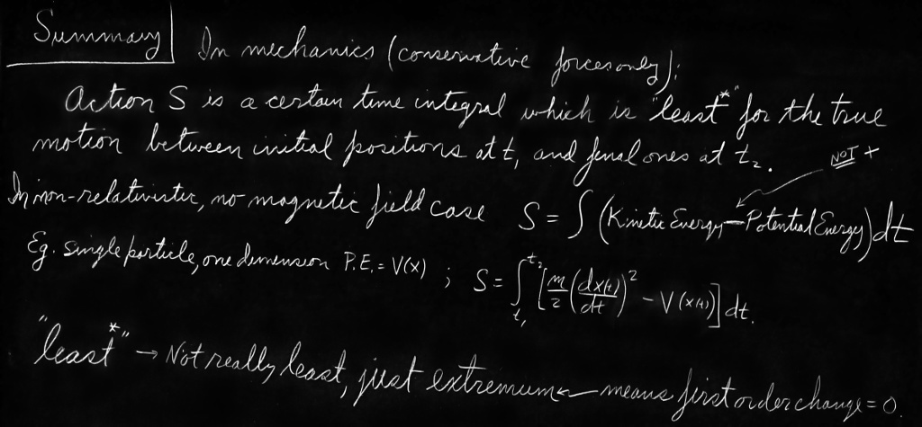
The cover picture is from Feynman’s lecture on ‘The Principle of Least Action’. Perhaps, it is the most interesting way to understand variational methods. If you would like to know more on the topic of variational methods, I recommend you check out the link in the picture credit!
References
- Bishop, C. M. (2007), Pattern Recognition and Machine Learning (Information Science and Statistics) , Springer
- Jordan, M.I., Ghahramani, Z., Jaakkola, T.S. and Saul, L.K., 1999. An introduction to variational methods for graphical models. Machine learning, 37(2), pp.183-233.